



ABC analysis is an inventory-management method that sorts every item you stock into three groups — A, B, and C — based on how much value each one represents, so you can put the most control on the stock that matters most. It’s built on the Pareto principle: roughly 20% of your items usually drive about 80% of your inventory value. ABC analysis makes that vital 20% visible, so you stop managing every SKU the same way and start managing by impact. This guide explains what ABC analysis is, how to do it step by step, a worked example, how to manage each category, and where it helps and falls short.
What Is ABC Analysis in Inventory Management?
ABC analysis is a way of classifying inventory into three tiers by value, so tight control goes to the items that carry the most value and less effort goes to the many low-value items. It applies the Pareto principle (the 80/20 rule) to a stockroom: a small share of items accounts for most of the money tied up in inventory, and a large share accounts for very little.
The point is prioritization. You have limited time for counting, forecasting, and reordering, so ABC analysis tells you where to spend it. Get the A items right and you control most of your inventory value; the C items can run on simple, low-effort rules.
What Are the A, B, and C Categories?
The three classes are A for the small group of high-value items, B for a moderate middle, and C for the long tail that carries very little — each assigned on its share of total inventory value:
| Class | Share of items | Share of value | How to manage |
|---|---|---|---|
| A — high value | ~10–20% | ~70–80% | Tight control, frequent counts, close forecasting |
| B — moderate value | ~20–30% | ~15–25% | Standard control, periodic review |
| C — low value | ~50–70% | ~5–10% | Simple rules, minimal effort, bulk reorders |
The exact percentages vary by business, but the pattern holds: a few A items dominate value, and a long tail of C items barely moves the needle.
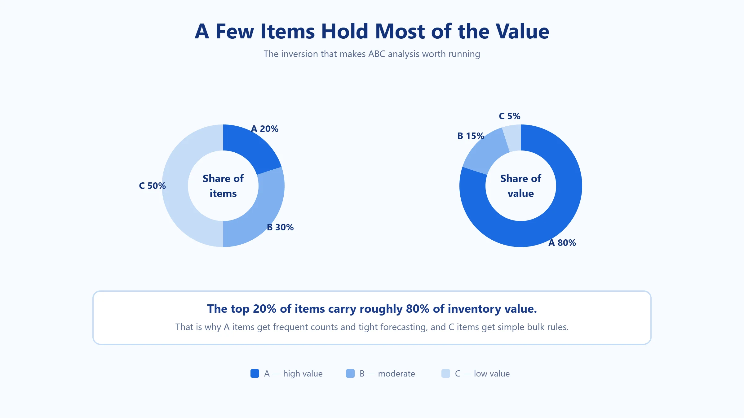
Published splits vary more than most guides admit. The Association for Supply Chain Management puts the A group at the top 10–20% of items accounting for 50–70% of sales volume, and the C group at the remaining 60–70% of items accounting for 10–30% — noticeably looser than the textbook 80/15/5. Treat any published split as a starting point and cut your own tiers against your own data.
How Do You Do an ABC Analysis? (Step by Step)
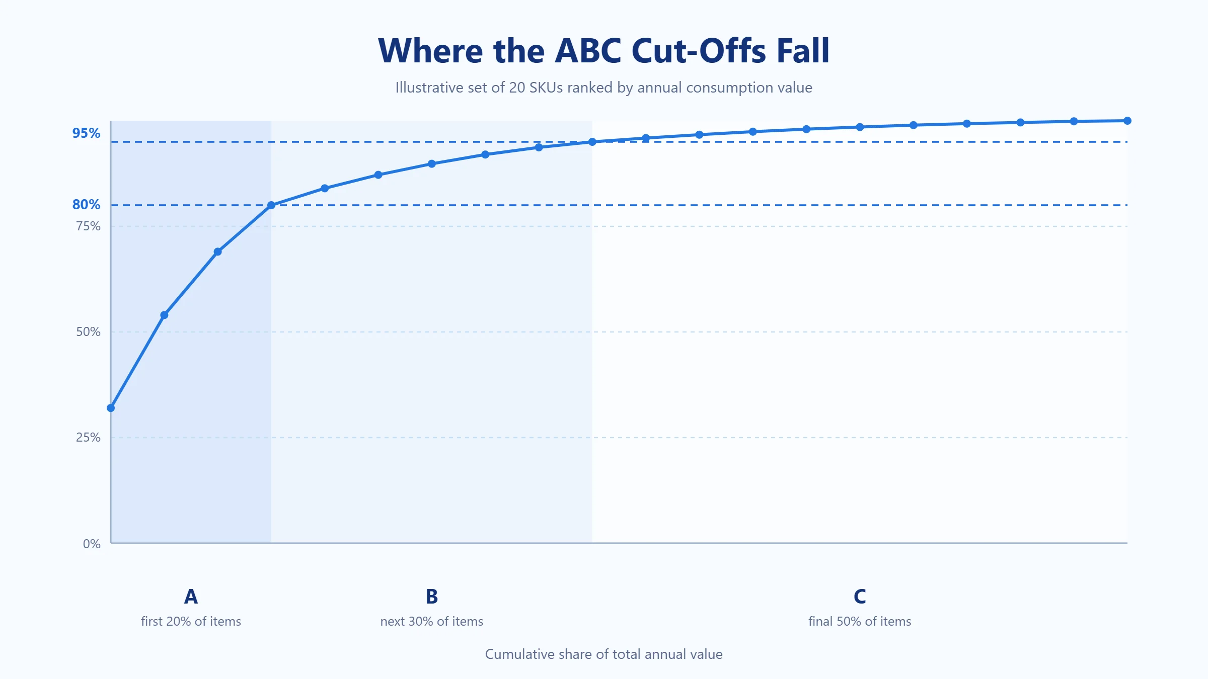
An ABC analysis runs in five steps: calculate each item’s annual value, rank every item from highest to lowest, add a cumulative percentage of total value, draw the cut-offs, then set control rules for each class. It works on a spreadsheet or straight from your inventory system:
- 1. Calculate each item’s annual value. Multiply annual usage (units sold or consumed per year) by cost or selling price per unit. This is the item’s annual consumption value.
- 2. Rank every item from highest to lowest annual value.
- 3. Add a running (cumulative) percentage of total value down the list.
- 4. Draw the cut-offs. Items making up roughly the first 80% of value are A, the next ~15% are B, and the final ~5% are C.
- 5. Set control rules for each class and review the classification a few times a year, since items move between tiers as demand changes.
What Does an ABC Analysis Look Like in Practice?
Three items are enough to show the shape: one expensive, slow-moving item carries most of the money, while a cheap item picked constantly carries almost none. Rank by annual value, then classify:
| Item | Unit cost | Annual usage | Annual value | Class |
|---|---|---|---|---|
| Motor | $500 | 200 | $100,000 | A |
| Control board | $120 | 150 | $18,000 | B |
| Bolt | $1 | 2,000 | $2,000 | C |
The bolt is used constantly but ties up little value, so it’s a C item you can reorder in bulk and count rarely. The motor ties up most of the money, so it’s an A item that needs tight control and frequent counts — even though far fewer move.
How Do You Run an ABC Analysis in a Spreadsheet?
Build five columns: SKU, annual usage, unit cost, annual value, and cumulative share of value. Sort descending by annual value, run a cumulative total down the list, and read the class off the cumulative percentage.
The mechanics, column by column:
- Annual value is usage multiplied by unit cost. This is the only calculated input that matters, and it is where most errors start — usage must cover a full year, and cost must be consistent across items.
- Sort descending on annual value. Everything after this depends on the ranking being right.
- Running total of annual value, then divide each running total by the grand total to get cumulative share.
- Class reads straight off cumulative share: at or below 80% is A, above 80% up to 95% is B, the rest is C. A nested conditional or a lookup table does it in one column.
- Item count check. Count how many rows fall into each class and compare against your share of items. If A is coming out at 40% of your SKUs, either the ranking is wrong or your inventory genuinely is not Pareto-shaped — both are worth knowing.
One practical caution: run it on a copy of the data with the date stamped in the filename. The classification is a snapshot, and comparing this quarter against last quarter is how you spot items migrating between tiers.
If the curve comes out flat, with no small group carrying most of the value, ABC will not help much — and that is a finding rather than a failure. Flat curves turn up in businesses with genuinely uniform product economics, where demand variability or criticality is the more useful lens to sort on.

How Should You Manage Each Category?
Each tier gets a different level of control: tight forecasting and frequent counts for A items, periodic review against standard reorder points for B, and bulk orders with minimal attention for C. The tiers only earn their keep when the control genuinely differs:
- A items: count them often (frequently, even weekly), forecast demand closely, hold safety stock carefully, and keep tight reorder control. A stockout or overstock here is expensive.
- B items: review periodically (monthly), use standard reorder points, and watch for items trending toward A or C.
- C items: keep it simple — bulk orders, larger safety stock (it’s cheap), and infrequent counts (quarterly). Don’t spend scarce management time here.
This is why ABC analysis pairs naturally with real-time inventory tracking and cycle counting: it tells you which items to count most often instead of shutting down for one big annual count.
Counting A items more often is the single biggest lever on inventory accuracy — the one warehouse KPI every other number depends on, and the first to fix when a scorecard stops making sense.
How Does ABC Compare With XYZ and VED Analysis?
ABC analysis sorts by value, but it isn’t the only lens. XYZ analysis sorts items by demand variability — X items sell steadily, Z items are erratic and hard to forecast. VED analysis (common in healthcare and maintenance) sorts by criticality — Vital, Essential, Desirable. Many operations combine methods, such as ABC-XYZ, to manage both value and predictability at once. ABC is the best starting point because value is the simplest, highest-impact way to prioritize.
What XYZ Analysis Adds
XYZ analysis classifies items by how predictable their demand is, which is the dimension ABC ignores. ASCM describes X items as ordered frequently, perhaps daily, with low and predictable demand variation; Y items as ordered less often, every few weeks or less, with more variation; and Z items as ordered infrequently and irregularly, with the most variation and the hardest forecasts.
The ABC-XYZ Matrix
Crossing the two gives nine cells, and the corners are where the decisions get interesting. Value tells you how much a mistake costs; variability tells you how likely you are to make one.
| X — steady demand | Y — some variation | Z — erratic demand | |
|---|---|---|---|
| A — high value | Never stock out. Tight reorder points, frequent counts | Hold safety stock and review forecasts closely | Often not stocked at all; order against demand |
| B — moderate | Standard reorder points, low effort | Periodic review, moderate safety stock | Consider make-to-order or supplier-held stock |
| C — low value | Bulk buy, count rarely | Bulk buy with generous safety stock | Buy as needed; the carrying cost is not worth planning |
ASCM makes the two extremes explicit: a company should never be out of stock on AX items, while AZ items likely would not be inventoried at all, because erratic demand on an expensive item is better met by ordering against a confirmed requirement than by holding stock and hoping.
How Does ABC Analysis Differ From EOQ?
ABC analysis tells you which items deserve attention; economic order quantity tells you how much of one to order at a time. They answer different questions and are used together rather than chosen between.
EOQ is a formula that balances ordering cost against carrying cost to find the order size with the lowest total cost. It works on one SKU at a time and needs reasonably steady demand to be meaningful. Running it across thousands of items is possible but rarely worth the effort, which is exactly where ABC comes in: classify first, then spend the modelling effort on the A items where a better order quantity actually moves money.
In practice the sequence is: rank by annual value, cut the tiers, then apply EOQ or a formal reorder policy to A items, simpler reorder points to B items, and flat bulk rules to C items. ABC decides where the effort goes; EOQ is one of the tools you spend that effort on.
What Are the Benefits and Limitations?
ABC analysis buys focus — management time and working capital aimed at the items that carry the value — at the cost of seeing only value, which misses items that are cheap to buy and expensive to run out of.
Benefits: ABC analysis focuses your time and cash on the items that matter, cuts carrying costs by right-sizing C-item stock, reduces stockouts on critical A items, and makes counting and forecasting far more efficient.
Limitations: it only looks at value, so it can miss a low-value item that’s critical to operations (a cheap part that halts production if it’s out). It also needs periodic re-running as demand shifts, and it doesn’t account for seasonality on its own. Pairing ABC with XYZ or a criticality check covers most of these gaps.
Where value alone is genuinely not enough, multi-criteria ABC weights two or three factors together — typically annual value, lead time and criticality — and ranks on the combined score. It is more work to maintain and harder to explain, so it earns its place in spare parts and regulated environments where a stockout has consequences beyond cost, and rarely anywhere else. Start with single-factor value ranking, and add a second factor only when you can name the items it would move.
How Often Should You Re-Run the Classification?
Re-run it quarterly for most operations, and monthly if demand moves fast or your product mix turns over quickly. A classification built once and left alone stops describing the business within a couple of quarters.
ASCM is direct about the risk: in a dynamic marketplace, sales can be erratic enough to push items between groups quickly and frequently, and if that goes unwatched the classification becomes obsolete — with knock-on effects on production, safety stock, service-level agreements and sales plans. The classification is not the deliverable; keeping it current is.
Two habits keep re-running cheap. First, do not let items flip on noise: if a SKU crosses a boundary by a fraction of a percent, leave it where it is until it holds the new position for two consecutive runs. Constant reclassification churns count schedules and reorder rules for no gain. Second, look at what moved rather than just the new list. An item climbing from C to A is a demand signal worth understanding before you simply tighten its controls.
How Do You Handle Seasonality and New SKUs?
Use a rolling twelve months of usage so seasonal peaks sit inside the window rather than distorting it, and hold new SKUs outside the classification until they have enough history to rank honestly.
Seasonality breaks ABC when the window is too short. Classify on a single quarter and a Christmas line looks like an A item in December and a C item in March, which produces a schedule that is wrong for most of the year. A trailing twelve-month window smooths that out. Where a business is seasonal end to end, run two classifications — one for peak, one for the rest of the year — rather than pretending one set of tiers fits both.
New SKUs have the opposite problem: no history at all. Ranking them on a few weeks of launch demand overstates them badly. Assign a provisional class from the item cost and the forecast, flag it as provisional, and let it fall into the normal classification at the next quarterly run once there is a full picture.
Common Mistakes When Running an ABC Analysis
The five that cost the most are ranking on the wrong measure, classifying once and never revisiting, ignoring criticality, treating the report as the outcome, and applying the tiers to counting but not to layout.
- Ranking on unit cost instead of annual value. An expensive item that sells twice a year ties up less money than a cheap one picked daily. Annual consumption value is usage multiplied by cost, and skipping the usage half is the most common error.
- Classifying once. Tiers built last year describe last year. Without a re-run cadence the schedule keeps protecting items that no longer matter.
- Ignoring criticality. A cheap fastener that halts a line is a C item by value and an A item by consequence. Pure value ranking cannot see that, which is why a criticality override or a VED check belongs alongside it.
- Stopping at the report. A classification nobody acts on changes nothing. The value is in the count schedule, the reorder rules and the slotting that follow from it.
- Using it for counting but not for layout. Many operations apply ABC to count frequency and then leave A items at the back of the building. Travel distance is where the labor cost actually sits.
ASCM adds a structural caution worth keeping in view: classifying items on one or two factors can simply be too simplistic. Value is the best single lens to start with, not the only one worth having.
How Does ABC Analysis Work With Your Warehouse System?
ABC analysis is far easier when your warehouse management system can rank items by value and flag their class automatically, rather than exporting to a spreadsheet each quarter. A good WMS uses the classification to drive automated slotting (A items near packing), count schedules, and reorder rules. Growing brands that outsource to a 3PL get this built in — the provider’s system applies ABC-style prioritization as part of running the operation.
Where Cura Resource Group applies this is slotting: A items go closest to pack-out, C items go to the back, and the classification gets revisited quarterly rather than set once. Most of the picking-time gain from ABC analysis comes from acting on it in the layout, not from producing the report.
Final Word
ABC analysis is one of the simplest, highest-return inventory methods there is. Sort your stock by annual value, give the A items tight control and the C items simple rules, and re-run it a few times a year. It won’t catch every nuance on its own, but as a way to focus limited time and cash on the inventory that matters most, nothing beats it for effort versus payoff.
Classifying items is the easy part; keeping the classes accurate as demand shifts is the work. That ongoing discipline is what inventory control covers — the counting cadence, the reorder rules, and the system that enforces both.
Want inventory managed by value, not guesswork?
Frequently Asked Questions
How does ABC analysis classify inventory?
ABC analysis classifies inventory into three groups by value: A items (high value, tight control), B items (moderate value), and C items (low value, simple control). It applies the Pareto 80/20 principle so you focus management effort on the small share of items that drive most of your inventory value.
How do you calculate ABC analysis?
Multiply each item’s annual usage by its cost to get its annual value, rank all items from highest to lowest, then add a cumulative percentage of total value. Items making up the first ~80% of value are A, the next ~15% are B, and the final ~5% are C.
What percentage is A, B, and C?
A commonly used split is roughly 20% of items driving about 80% of value as A, the next 30% of items driving about 15% as B, and the remaining 50% driving the last 5% as C. Treat those as starting points and recalculate against your own sales data.
What is the difference between ABC and XYZ analysis?
ABC classifies items by consumption value — how much money moves through each SKU. XYZ classifies by demand variability — how predictable that consumption is. Used together they are more useful than either alone, because a high-value item with erratic demand needs different safety stock to a high-value item with steady demand.
What are the limitations of ABC analysis?
ABC analysis only considers value, so it can overlook a low-value item that is operationally critical. It also needs periodic re-running as demand changes and doesn’t handle seasonality alone. Pairing it with XYZ or a criticality (VED) check addresses most gaps.
What is the difference between ABC analysis and EOQ?
ABC analysis decides which items deserve management attention; economic order quantity decides how much of a single item to order at a time. They are complementary: classify with ABC first, then spend the EOQ modelling effort on the A items where a better order quantity actually saves money.
How do you do an ABC analysis in Excel?
Build columns for SKU, annual usage, unit cost, annual value and cumulative share of value. Multiply usage by cost, sort descending on annual value, run a cumulative total, divide each running total by the grand total, then read the class off cumulative share at the 80% and 95% boundaries.
How often should ABC classification be updated?
Quarterly suits most operations, monthly where demand or product mix moves quickly. ASCM warns that erratic sales can push items between groups fast enough for a stale classification to become obsolete, so the cadence matters more than the precision of the original cut.
Sources & Further Reading
- Association for Supply Chain Management, The XYZs of Inventory Management — ABC and XYZ classification, published class ranges, and the limitations of value-only ranking.